How To Use Gps Data Into An App

How tracking apps analyse your GPS data: a hands-on tutorial in Python

Sport tracking applications and the social networks accompanying them are all over the place nowadays. Everyone wants to make the biggest or the fastest effort on apps like Nike+ Run or Strava. But have you ever wondered where all these fancy statistics come from, or how they are calculated?

Let's start with explaining how your phone knows where you are, or more precisely, how the GPS receiver in your phone knows where you are. The Global Positioning System (GPS) is a satellite-based radionavigation system owned by the United States government.

It is a gl o bal navigation satellite system that provides geolocation and time information to a GPS receiver anywhere on the planet where there is an unobstructed line of sight to four or more GPS satellites. Your phone's receiver's location is usually converted to latitude, longitude and altitude, accompanied by a time stamp and stored as a gpx-file (more about the file format below).

In this tutorial we'll extract, munge and analyse the gpx data of one single route in a Jupyter Notebook with Python. We'll start with extracting the data from the gpx-file into a convenient pandas dataframe. From there we'll explore the data and try to replicate the stats and graphs that the interface of our favorite running application provides us with.

Getting the data

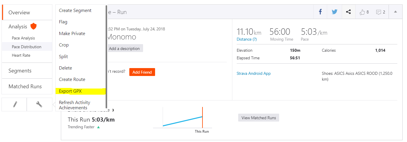
Most of the populair tracking apps allow you to download your effort as a gpx-file. In this tutorial, we download an eleven kilometer run from Strava. The gpx-file, short for GPS Exchange Format, can usually be obtained by clicking on export. The screenshot below shows you where you can download your gpx-file in Strava. You can download the file used in this article here.

Gpx is an XML-schema designed as a common GPS data format for software applications. It can be used to describe waypoints, tracks, and routes. This also means that all the code below can be used to run on any GPS data, provided that you take into account the speed and type of movement.

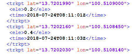
First, it's important to understand the structure of our gpx-file. After opening the file into any text editor (Notepad ++ here), you should get an XML-file with a lot of entries like the ones below. Note that each trackpoint consists of four values: latitude, longitude, elevation or altitude and a timestamp. These four values will be the backbone of our analysis.

Loading the data

Now, we want to load our gpx data into a pandas dataframe. There is no direct way to do this, so we'll have to use the gpxpy library to assist us. While we're importing modules, you might want to make sure that you have the following libraries installed as well: matplotlib, datetime, geopy, math, numpy, pandas, haversine and plotly (optional). Download the libraries, and make sure the following code can run successfully.

          import gpxpy
import matplotlib.pyplot as plt
import datetime
from geopy import distance
from math import sqrt, floor
import numpy as np
import pandas as pd
import plotly.plotly as py
import plotly.graph_objs as go
import haversine

Loading the gpx data into Python is as easy as opening the file in read mode and parsing it into a new variable.

          gpx_file = open('my_run_001.gpx', 'r')
gpx = gpxpy.parse(gpx_file)

Take a look at the new object and note that it's a GPX object that consists of a list of GPXTrack objects. The GPXTrack objects on their turn exist of a list of GPXTrackSegment objects, which on their turn exist of GPXTrackPoints. These points are the four-value data points we're interested in. They can be accessed with the longitude, latitude, elevation and time attributes.

Before consuming the data, it's important to check how your data is divided between these objects. You can do this by checking the length of the tracks, segments and points list.

          len(gpx.tracks)
len(gpx.tracks[0].segments)
len(gpx.tracks[0].segments[0].points)

In our example the length of both tracks and segments is 1. This means all the data is concentrated in the points attribute of the first segment of the first track. It makes sense to create a new variable that points directly to the list of data points.

          data = gpx.tracks[0].segments[0].points

Take a look at your start point and end point and make sure everything makes sense (i.e. start time < end time, start elevation = end elevation, etc…). If not, there might be something wrong with your data, or you might have forgotten about some tracks or segments.

          ## Start Position
start = data[0]
## End Position
finish = data[-1]

Once you've located all your data, pouring everything into a dataframe is easy. Just create an empty dataframe and iterate through all the data points while adding them to the dataframe.

          df = pd.DataFrame(columns=['lon', 'lat', 'alt', 'time'])          for point in data:
            df = df.append({'lon': point.longitude, 'lat' : point.latitude, 'alt' : point.elevation, 'time' : point.time}, ignore_index=True)

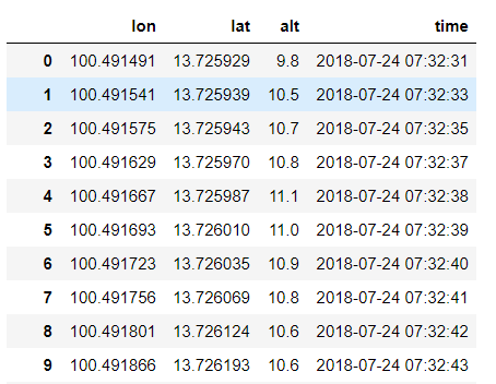
The head of the dataframe should look like this:

Note that the time interval between data points is supposed to be one second (for Strava, you can change this in your settings). Unfortunately, my device can't always provide the GPS-data, due to connectivity problems. In case of such a failure the data point is skipped (without an error of any kind) and the application will collect the data at the next time interval. It is important to keep this in mind for further analysis and not to assume that the interval between all points is the same.

Plotting the data

Now we have our data loaded, we can start exploring it with plotting some basic graphs. The two easiest ones are a 2d map (longitude vs latitude) and our elevation gain during our activity (altitude vs time). Comparing these plots with the ones from our app, we can see we did a pretty good job, so far.

          plt.plot(df['lon'], df['lat'])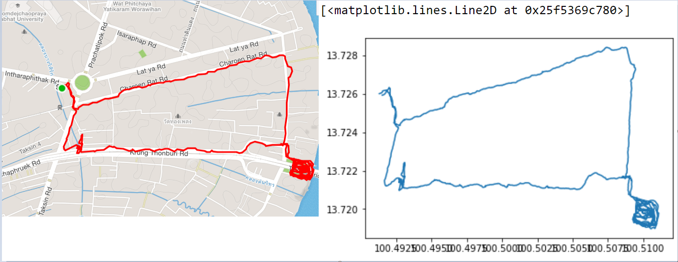

          plt.plot(df['time'], df['alt'])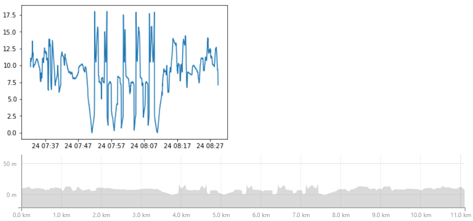

If we want to get really fancy, we can plot an interactive 3d line of our data with plotly. Although it's debatable if this plot adds any analytical value to our story, it always feels good to look at your tremendous effort from another angle. If you haven't used plotly before, don't forget to create an account on plot.ly and set your username and API-key in the credentials-file.

          _data = [go.Scatter3d(x=df['lon'],            
            y=df['lat'], z=df['alt'], mode='lines')]          py.iplot(_data)

If you want to learn how to overlay your plot on Google Maps, take a look a this tutorial about gmplot.

Transforming the data

While we've done pretty good so far, we are still missing a few key values, such as distance and speed. It doesn't seem too hard to calculate these two, but there are a few trap-holes. The first one is that we have to take into account that the distance between two LL-points (longitude, latitude) isn't a straight line, but spherical.

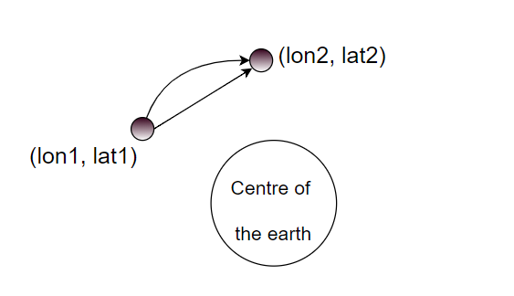
Spherical distance vs Euclidean distance

There are two main approaches to calculate the distance between two points on a spherical surface: the Haversine distance and the Vincenty distance. The two formulas take a different approach on calculating the distance, but this is outside the scoop of this article. You can find more information on their Wikipedia pages: Haversine Formula Wiki and Vincenty Formula Wiki.

The next issue is that we might want to take into account the elevation gain or loss in our calculations. The easiest way to do this, is to calculate the spherical 2d distance and then use the Euclidean formula to add the third dimension. The formula below shows this last step.

distance_3d = sqrt(distance_2d**2 + (alt2 — alt1)**2)

Now we have all the theoretical background needed, we can start implementing the formula in our code. For convenience, we leave our dataframe for what it is, and iterate through all the data points just like we did before. We create a list for every possible implementation of our distance formula (Haversine or Vincenty and 2d or 3d) and add the total distance to the end of the list for every data point.

While we're looping through the data points, we also create a list for the altitude difference, time difference and distance difference between all the consecutive data points.

          alt_dif = [0]
time_dif = [0]
dist_vin = [0]
dist_hav = [0]
dist_vin_no_alt = [0]
dist_hav_no_alt = [0]
dist_dif_hav_2d = [0]
dist_dif_vin_2d = [0]          for index in range(len(data)):
            if index == 0:
            pass
            else:
            start = data[index-1]                      stop = data[index]
                                  distance_vin_2d = distance.vincenty((start.latitude, start.longitude), (stop.latitude, stop.longitude)).m
                                dist_dif_vin_2d.append(distance_vin_2d)                      distance_hav_2d = haversine.haversine((start.latitude, start.longitude), (stop.latitude, stop.longitude))*1000
                    dist_dif_hav_2d.append(distance_hav_2d)                      dist_vin_no_alt.append(dist_vin_no_alt[-1] + distance_vin_2d)
                                  dist_hav_no_alt.append(dist_hav_no_alt[-1] + distance_hav_2d)
                                  alt_d = start.elevation - stop.elevation
                                  alt_dif.append(alt_d)
                                  distance_vin_3d = sqrt(distance_vin_2d**2 + (alt_d)**2)
                                  distance_hav_3d = sqrt(distance_hav_2d**2 + (alt_d)**2)
                                  time_delta = (stop.time - start.time).total_seconds()
                                  time_dif.append(time_delta)
                                  dist_vin.append(dist_vin[-1] + distance_vin_3d)
                                  dist_hav.append(dist_hav[-1] + distance_hav_3d)

For further convenience, we can pour the data in our previously created dataframe.

          df['dis_vin_2d'] = dist_vin_no_alt            
df['dist_hav_2d'] = dist_hav_no_alt
df['dis_vin_3d'] = dist_vin
df['dis_hav_3d'] = dist_hav
df['alt_dif'] = alt_dif
df['time_dif'] = time_dif
df['dis_dif_hav_2d'] = dist_dif_hav_2d
df['dis_dif_vin_2d'] = dist_dif_vin_2d

Check the results with the following print command.

          print('Vincenty 2D : ', dist_vin_no_alt[-1])
print('Haversine 2D : ', dist_hav_no_alt[-1])
print('Vincenty 3D : ', dist_vin[-1])
print('Haversine 3D : ', dist_hav[-1])
print('Total Time : ', floor(sum(time_dif)/60),' min ', int(sum(time_dif)%60),' sec ')

The output should look like this. Let's also compare our results with the statistics our running app shows us.

There are a few things to notice. Firstly, all our total distance calculations — especially the 2d ones — seem to be a good approximation of the distance our app calculated for us. Secondly, the total activity time agrees completely with our calculations, but the moving time seems to be different.

This can signify that whenever the distance between two data points was too small, the app has stopped the moving time, but still took the distance into account, this can be realistic when we have to slow down and stop for a traffic light, for example.

In this scenario our 2d calculations are right and the we can conclude the app doesn't take elevation into account. This is indeed confirmed by a blogpost from the app company.

A flat surface is assumed, and vertical speed from topography is not accounted for. — Strava

Worrisome? Not really. The difference between the distance proposed by the app and our maximum 3d estimate is only 61m (0.55%). This means that the total round-down for a 100km run (or ride) would by around 600m. Note that this difference will increase if you undertake more altitude-intense activities (mountain biking or hiking).

Let's see if we can figure out which threshold Strava uses to stop the timer (and therefore boost our average speed). To do so, we need to create a new variable that calculates our movement in meters per second (and not just movement per data point, hence why we created the time difference variable). Let's do this for our haversine 2d distance, since that's the closest approximation of the distance proposed by the app.

          df['dist_dif_per_sec'] = df['dis_dif_hav_2d'] / df['time_dif']

With this new variable we can iterate through a bunch of thresholds, let's say between 50 cm and 1 meter, and try to figure out which one adds up to a timer time-out closest to 51 seconds.

          for treshold in [0.5, 0.6, 0.7, 0.8, 0.9, 1]:
            print(treshold, 'm', ' : Time:',            
            sum(df[df['dist_dif_per_sec'] < treshold]['time_dif']),
            ' seconds')

Your Notebook should print something like this.

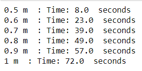
We can therefore conclude that if the movement per seconde was less than 80 centimeters, the application didn't consider it as a movement and stopped the timer. This seems very reasonable, since 80 centimeters per second is about 2.9 km per hour, a speed far below most people their walking pace.

While talking about pace, we might as well calculate the speed for every data point. First, we create a new column in our dataframe named speed. This new variable is calculated by dividing the distance traveled in meters by the time it took in seconds, and then converted to km/h.

          df['spd'] = (df['dis_dif_hav_2d'] / df['time_dif']) * 3.6

Next, we filter out all the data where the movement per second is larger than 90 centimeters (see section above for the reason).

          df_with_timeout = df[df['dist_dif_per_sec'] > 0.9]

Then we calculate the weighted average speed and convert it to minutes and second per kilometer (a metric widely used by runners).

          avg_km_h = (sum((df_with_timeout['spd'] *            
            df_with_timeout['time_dif'])) /            
            sum(df_with_timeout['time_dif']))          print(floor(60 / avg_km_h), 'minutes',
            round(((60 / avg_km_h - floor(60 / avg_km_h))*60), 0),
            ' seconds')

This results in an average speed of 5 minutes and 3 seconds per kilometer, exactly the same speed as proposed by our app. Let's also draw a plot of our speed. Drawing a data point for every second would be to fine-grained, so we'll draw an average speed data point for every 10 seconds.

Therefore, create a new variable that rounds down the cumulative sum of our time difference to 10 seconds, and plot the aggregated speed against it.

          df['time10s'] = list(map(lambda x: round(x, -1)
            , np.cumsum(df['time_dif'])))
plt.plot(df.groupby(['time10s']).mean()['spd'])

The result is a smooth line plot where we can see the speed in km/h against the time in seconds.

The last metric we'll take a closer look at, is the elevation gain. According to the apps documentation, the cumulative elevation gain refers to the sum of every gain in elevation throughout an entire trip. This means we should only take into account the positive altitude gain.

We can write a simple function and map it over our altitude difference column of our dataframe.

          def positive_only(x):
            if x > 0:
            return x
            else:
            return 0          pos_only = list(map(positive_only, df['alt_dif']))          sum(pos_only)

The sum is about 237 meters, pretty far from what our app told us we elevated (150 m). Taking a closer look to the altitude difference we can see that it's measured down to 10 centimeters.

In case of running this could be jumping up and down a pavement, or scratching your head with your phone in your hand. It would make sense to round the numbers down to 1 meter. We can do this by mapping a lambda function over our previous results.

          sum(list(map(lambda x: round(x,0) , pos_only)))

The new result is 137m, pretty close to the elevation proposed by the app. Knowing this, we should also recalculate our 3d distances with these new elevation values in place. Without doing the calculations, we know that the total distance will go down and close in on the 2d distance. This makes the not taking into account of the altitude gain in total distance even more justified.

Something to think about

I'll round up this article with a revelation about the elevation gain: I didn't gain any altitude during the actual run (except for a few minor staircases). There is even more, my phone, just like most lower market phones, does not have a barometer.

A barometer is an instrument measuring atmospheric pressure, used especially in forecasting the weather and determining altitude. But how did Strava determine our altitude then? The answer is Strava's Elevation Basemap.

It is created using data from the community. By collecting the barometric altimeter measurements (from devices with a barometer) from any activity uploaded to Strava in the past, they are able to build a global elevation database.

For now the Basemap isn't reliable enough and doesn't cover enough of the world. But if they can make it more reliable in the future, they might be able, in combination with 3d calculations and a more complicated model on elevation gain, to provide all you sporters out there with even more accurate statistics.

What's next?

In a follow-up of this article we'll visualize all the data obtained during this tutorial with another hot kid on the block: QlikView.

— Please feel free to bring any inconsistencies or mistakes to my attention in the comments or by leaving a private note. —